A Simplified Introduction to Computational Fluid Dynamics
To analyze fluid behavior, knowledge of its velocity and pressure throughout the domain is essential. The governing equations of fluid flow are the equations of conservation of mass and momentum, which are commonly referred to as the Navier-Stokes equations. The Navier-Stokes equations are nonlinear and without applying simplifying assumptions, mathematics is unable to solve them. Numerical methods are used to analyze these equations. Computational Fluid Dynamics (CFD) is a science that uses simplifying assumptions to solve these equations through computers.
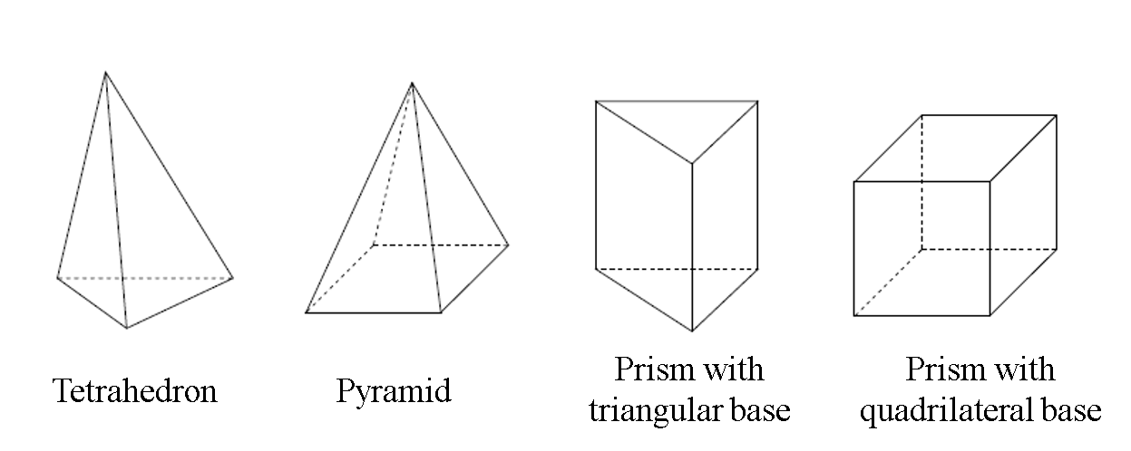
The main step in CFD flow simulation is mesh/grid generation. The basic principle is that the volume or surface under calculation is divided into very small sections like Figure 1. The choice of these shapes depends greatly on the type of physical problem and flow conditions. The higher the quality of meshing where the edges of each generated shape are equal, the better the mesh quality becomes. The quality of the created grid has a very significant impact on the accuracy and stability of the solution. Therefore, great accuracy and patience must be applied to generate a suitable mesh, because under conditions where the mesh does not have suitable quality, converging the solution will be very difficult.
Figure1-Meshing Shape
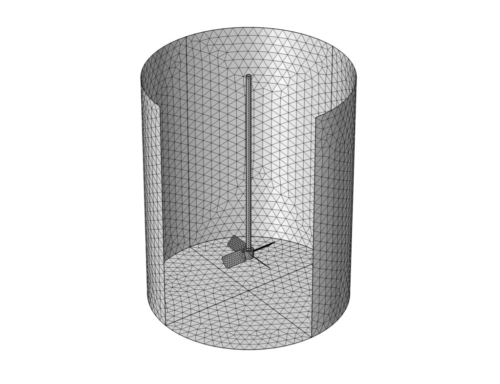
Figure 2 illustrates the meshing of a tank being studied. It is evident from the figure that in order to generate a high-quality mesh, a large number of grid cells is required, resulting in an extremely fine mesh. However, it is important to acknowledge that a computer capable of handling such a large number of elements may not always be readily available, or the computation time might become excessively long and tedious. Consequently, creating an accurate and high-quality mesh poses a significant challenge in problem-solving, heavily relying on the experience of the Computational Fluid Dynamics (CFD) user.
Figure2-Meshing A tank
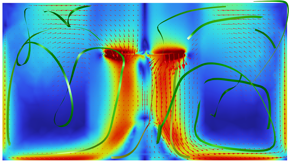
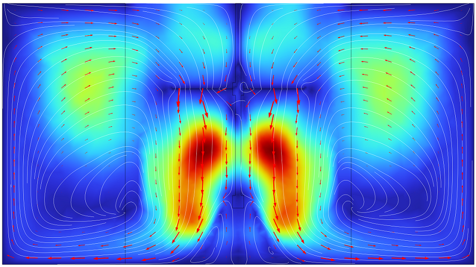
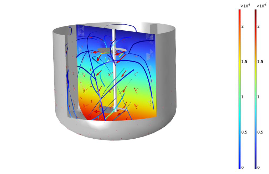
After generating an appropriate mesh and solving the governing equations at the generated nodes, when the difference in solution values between adjacent nodes becomes less than 0.0001, the results converge, and velocity and pressure contours are obtained as the output. Examples of these contours can be observed below: